Bayesian Learning Exercises 3 notes

Lecture 7, Slide 21: Gibbs sampling for mixture distributions

Prior and notation

Prior:

Conjugate prior for $(\mu_j,\sigma_j^2)$, see Slide 16.

Here $\pi$ is the mixing probability for component 1. The latent indicator $I_i$ records which mixture component generated observation $x_i$, so the Gibbs sampler alternates between updating the component parameters and updating these hidden labels.

Define:

Gibbs sampling steps

This $\theta_i$ is the posterior probability that observation $x_i$ belongs to component 1, after comparing how well both mixture components explain the same observation.

1. Gibbs step for an indicator variable

Problem

Show that the full conditional posterior of $I_i$ on Lecture 7, Slide 21, is correct.

Handwritten solution

Show that

where

Model

The normal density model is

and the prior probability of the indicator is

Conditional independence

In the Gibbs sampler, we sample

and then sample

Therefore,

where $\cdot$ denotes $\mu_1,\mu_2,\sigma_1^2,\sigma_2^2$.

The important simplification is that once the parameters are fixed, each observation only needs its own $x_i$ to update its own label. The other observations affect $I_i$ only indirectly through the current parameter values.

Fact 1:

Fact 2:

Full conditional

To derive the full conditional, we keep only the terms that depend on $I_i$. Constants that are the same for $I_i=1$ and $I_i=2$ disappear into the normalizing constant.

By Bayes' theorem,

Hence,

so

Since $I_i\in\{1,2\}$, the full conditional is Bernoulli after normalization. Find the normalizing constant from

Thus,

and

Therefore,

Intuitively, the numerator is the unnormalized weight for component 1. The denominator adds the two possible component weights, so the ratio turns the weight into a probability.

2. Frequentist vs Bayesian

Problem

2(a)

Let $x_1,\ldots,x_n\mid\theta\stackrel{iid}{\sim}\operatorname{Uniform}\left(\theta-\frac12,\theta+\frac12\right)$. Let $\hat{\theta}=\bar{x}=\frac1n\sum_{i=1}^{n}x_i$ be an estimator of $\theta$. Derive an expression for the repeated sampling variance of $\hat{\theta}$.

2(b)

Derive the posterior distribution for $\theta$ assuming a uniform prior distribution.

Hint: Here it is absolutely crucial to think about the support for the data distribution. Once you have observed some data, some values are no longer possible. I strongly suggest that you plot some imaginary data on the real line and plot the data distribution in the same graph for some made-up values of $\theta$. Just to make you think in the right direction.

2(c)

Assume that you have observed three data observations: $x_1=1.13$, $x_2=2.1$, $x_3=1.38$. What do we conclude from a frequentist perspective about $\theta$? What do we conclude from a Bayesian perspective about $\theta$? Discuss.

Handwritten solution

2(a)

Let

Let

Then

This is a repeated sampling variance: it describes how much $\bar{x}$ would vary if we repeatedly collected new samples of size $n$ from the same model. It is not a posterior variance for $\theta$.

2(b)

Assume a flat uniform prior:

The model density is

The posterior is

Within the support allowed by all observations, this is proportional to 1, so $\theta\mid\vec{x}$ is uniform on the feasible interval.

The key point is the support. A candidate value of $\theta$ is possible only if every observed $x_i$ lies inside the interval centered at $\theta$ with width 1. Values of $\theta$ outside this feasible interval get likelihood zero.

Determine the bounds for $\theta\mid\vec{x}$.

Given

let

At the same time,

Therefore,

which implies

Thus,

and

2(c)

Given

the frequentist estimate is

The Bayesian posterior is

The frequentist estimate summarizes the center of the observed data through $\bar{x}$. The Bayesian posterior instead uses the model support to rule out impossible values of $\theta$, leaving only a short interval of feasible values.

3. The posterior becomes more normal

Problem

3(a)

Let $x_1,\ldots,x_n\mid\theta\stackrel{iid}{\sim}\operatorname{Bern}(\theta)$ and let $\theta\sim\operatorname{Beta}(\alpha,\beta)$ a priori. Find the posterior mode of $\theta$.

3(b)

Approximate the posterior distribution of $\theta$ by a normal distribution.

3(c)

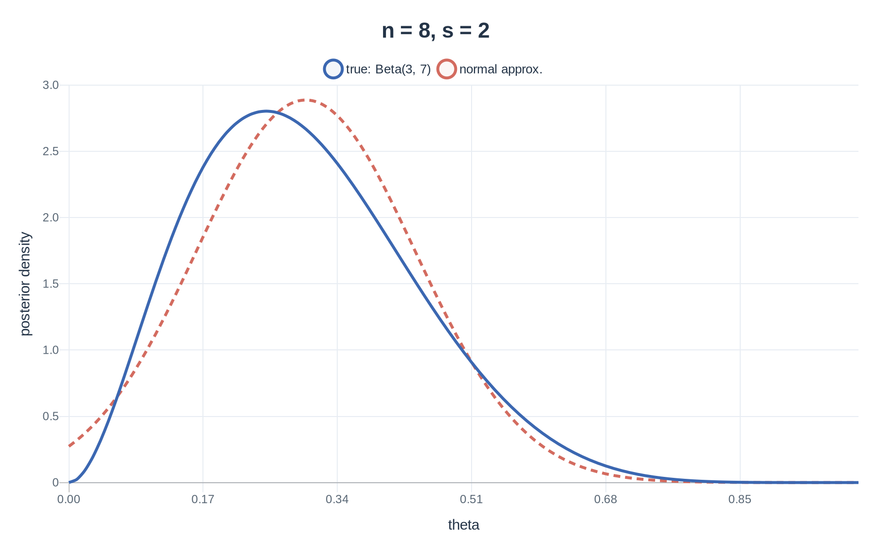
Assume now that you have the data $n=8$ and $s=2$. Plot the true posterior distribution and the normal approximation in the same graph. Assume a uniform prior for $\theta$.

3(d)

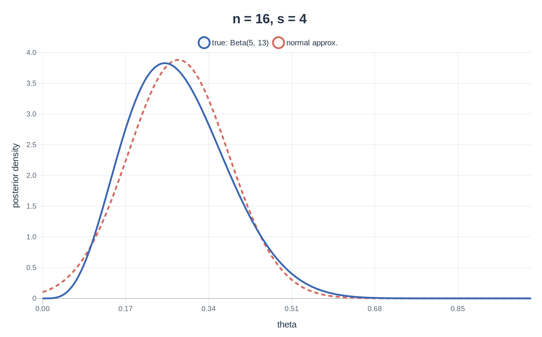
Redo the previous exercise, but this time with twice the data size: $n=16$ and $s=4$. What do you conclude?

Handwritten solution

3(a)

Find the stationary point:

Let $s$ be the number of successes and $f=n-s$ be the number of failures. Then

Expanding gives

so

Therefore,

This is the posterior mode, not necessarily the posterior mean. It is the value of $\theta$ where the posterior density is highest, assuming the mode is inside the interval $(0,1)$.

3(b)

Approximate the posterior by

where $J_{\vec{x}}(\hat{\theta})$ is the negative Hessian of the log posterior evaluated at $\hat{\theta}$.

This is a Laplace approximation. Near its mode, a smooth log posterior can be approximated by a quadratic curve; exponentiating that quadratic gives a normal density. The inverse curvature controls the approximate variance.

Also,

Substitute $\hat{\theta}$ and $1-\hat{\theta}$ into $J_{\vec{x}}(\hat{\theta})$:

Therefore,

Hence,

where

and

As the sample size increases while the success proportion stays similar, the posterior becomes more concentrated and the normal approximation usually improves. This is the sense in which the posterior becomes more normal.

3(c) Plot: $n=8, s=2$

For the plots, use the moment-matched normal approximation from the handwritten note:

With a uniform prior, $\alpha=\beta=1$, so for $n=8$ and $s=2$ we have

3(d) Plot: $n=16, s=4$

Doubling the data while keeping the same success proportion gives

The second posterior is more concentrated and the normal curve tracks the true posterior more closely. This supports the conclusion that, as the amount of data increases, the posterior tends to look more normal.